Calibrated Ice Thickness Estimate for All Glaciers in Austria
 Kay Helfricht
 Matthias Huss
 Andrea Fischer
 Jan-Christoph Otto
- 1Institute for Interdisciplinary Mountain Research, Austrian Academy of Sciences, Innsbruck, Austria
- 2Department of Geosciences, University of Fribourg, Fribourg, Switzerland
- 3Laboratory of Hydraulics, Hydrology and Glaciology (VAW), ETH Zurich, Zurich, Switzerland
- 4Department of Geography and Geology, University of Salzburg, Salzburg, Austria
Knowledge on ice thickness distribution and total ice volume is a prerequisite for computing future glacier change for both glaciological and hydrological applications. Various ice thickness estimation methods have been developed but regional differences in fundamental model parameters are substantial. Parameters calibrated with measured data at specific points in time and space can vary when glacier geometry and dynamics change. This study contributes to a better understanding of accuracies and limitations of modeled ice thicknesses by taking advantage of a comprehensive data set of in-situ ice thickness measurements from 58 glaciers in the Austrian Alps and observed glacier geometries of three Austrian glacier inventories (GI) between 1969 and 2006. The field data are used to calibrate an established ice thickness model to calculate an improved ice thickness data set for the Austrian Alps. A cross-validation between modeled and measured point ice thickness indicates a model uncertainty of 25–31% of the measured point ice thickness. The comparison of the modeled and measured average glacier ice thickness revealed an underestimation of 5% with a mean standard deviation of 15% for the glaciers with calibration data. The apparent mass balance gradient, the primary model parameter accounting for the effects of surface mass balance distribution as well as ice flux, substantially decreases over time and has to be adjusted for each temporal increment to correctly reproduce observed ice thickness. This reflects the general stagnation of glaciers in Austria. Using the calibrated parameter set, 93% of the observed ice thickness change on a glacier-specific scale could be captured for the periods between the GI. We applied optimized apparent mass balance gradients to all glaciers of the latest Austrian glacier inventory and found a volume of 15.9 km3 for the year 2006. The ten largest glaciers account for 25% of area and 35% of total ice volume. An estimate based on mass balance measurements from nine glaciers indicates an additional volume loss of 3.5 ± 0.4 km3 (i.e., 22 ± 2.5%) until 2016. Relative changes in area and volume were largest at glaciers smaller than 1 km2, and relative volume changes appear to be higher than relative area changes for all considered time periods.
Introduction
Climate observations as well as climate scenarios reveal a rise of temperatures around the globe (IPCC, 2014), with almost twice the global rate in the Alps, and, for example, in Austria (Auer et al., 2007; APCC, 2014). At the same time, historically unprecedented glacier retreat can be observed (WGMS, 2015; Zemp et al., 2015). This raises the awareness of severe implications for coastal regions but also for water resource management in mountain regions, for river ecosystems and for potential natural hazards originating from glacial and periglacial environments (e.g., Kaser et al., 2010; Haeberli et al., 2014; Marzeion et al., 2014; Radić and Hock, 2014).
Knowledge of the spatial ice thickness distribution in glacierized mountain regions and the elevation of the bedrock underneath the glaciers represents an essential basis for numerous applications in climate impact research. For example, assessments of anticipated sea-level rise caused by glacier mass loss importantly depend on initial ice volume estimates (e.g., Marzeion et al., 2012; Radić et al., 2014; Huss and Hock, 2015). Most regional and global glacier models estimate initial ice volume applying simple volume-area scaling relations (e.g., Bahr et al., 1997; Radić and Hock, 2010; Bahr et al., 2015) on the basis of global glacier inventories (GI) (e.g., Pfeffer et al., 2014). However, volume-area scaling only provides average ice thickness for each glacier and cannot take into account a number of parameters with major impact on glacier volume, such as surface slope or the climatic regime affecting mass balance. Recently, a number of approaches with different levels of complexity have been developed to infer ice thickness distribution by relying on physically based models (e.g., Clarke et al., 2009; Farinotti et al., 2009b; Morlighem et al., 2011; Huss and Farinotti, 2012; Li et al., 2012; Linsbauer et al., 2012; van Pelt et al., 2013; Frey et al., 2014; Maussion et al., 2018). The Ice Thickness Models Intercomparison Experiment (ITMIX; Farinotti et al., 2017) has assessed the skill of seventeen different approaches to reproduce observed thickness for various glacier types around the globe. A considerable variability among the individual approaches has been found when not calibrating against withheld ice thickness measurements. Huss and Farinotti (2012) presented the first estimate of ice thickness distribution for all roughly 200’000 individual glaciers on Earth allowing the application of a global glacier-specific model for future sea-level rise and the response of glacier runoff (Huss and Hock, 2015, 2018).
Furthermore, knowledge on spatial ice thickness distribution is also important for assessing bedrock overdeepenings that could potentially be filled with water after glacier retreat, thus forming proglacial lakes, which might become relevant in terms of natural hazards but could also form important sediment traps (Haeberli et al., 2016). Proglacial lakes are reported to grow in number and size in several mountain ranges of the globe following a rise in temperature. This indicates their increasing significance within mountain landscapes (Mergili et al., 2013; Wang et al., 2013; Emmer et al., 2016; Buckel et al., 2018). Several studies have also modeled the number and volume of potential new lakes forming after glacier melt in the future and have pointed out the significance of these new landforms for some mountain regions (e.g., Linsbauer et al., 2012; Haeberli and Linsbauer, 2013; Linsbauer et al., 2016; Colonia et al., 2017).
However, insufficient observations, process understanding, and modeling capacities still hamper accurate prediction of future changes in the cryosphere (Hock et al., 2017). Additional effort is needed to develop and calibrate ice thickness models for deriving accurate estimates of ice volume on a regional scale, as well as for inferring detailed bedrock topographies for impact studies.
Alpine glaciers, with a high density of observations over many decades, provide an excellent basis for improving process understanding and models. For Austria, three GI quantify area and volume loss at more than 800 glaciers (GI 1: Patzelt, 1978, 1980; GI 2: Lambrecht and Kuhn, 2007; GI 3: Fischer et al., 2015b; all GIs in shapefile format: Fischer et al., 2015a). What’s more, glacier mass loss has accelerated (Abermann et al., 2010) and, at the same time, glacier ice flow has decelerated (e.g., Span et al., 1997; Stocker-Waldhuber et al. unpublished). A few estimates of the total glacier volume in Austria exist from regional studies. Patzelt (1978) estimated a volume of 21 km3 for all glaciers of the first Austrian Glacier Inventory (GI 1) in 1969, which is equal to a mean ice thickness of 40 m. Lambrecht and Kuhn (2007) used observed ice volume changes for calibrating a volume-area scaling relationship specific to Austrian glaciers and found a volume of 22.8 km3 for GI 1 and of 17.7 km3 for GI 2. Fischer and Kuhn (2013) constructed ice volumes for a set of 64 glaciers in Austria, which represent 50% of the total glacier area of GI 2 by extrapolating ground penetrating radar (GPR) point measurements manually. For the investigated glaciers, they found a volume of 11.9 ± 1.1 km3, equal to a mean ice thickness of 50 ± 3 m. Whereas Lambrecht and Kuhn (2007) used a bulk estimation method and did not consider variations in the volume-area scaling relation between individual glaciers, the assessment by Fischer and Kuhn (2013) is based on glacier-specific ice thickness measurements. So far, however, there is no comprehensive estimate of Austria’s glacier volume based on an approach including all existing ice thickness measurements and a consistent and physically based extrapolation to all unmeasured glaciers. A more sophisticated estimation of the present ice volume will be the basis for regional as well as global studies on glacier retreat and related hydrological impacts.
Many models for computing spatially distributed ice thickness that account for mass conservation include parameters controlling ice flow flux (see Farinotti et al., 2017, for a review). Whereas parameters like the flow rate factor can be assumed to remain constant for temperate glaciers (e.g., Gudmundsson, 1999), parameters prescribing surface mass balance distribution, and, hence, cumulative mass fluxes along the glacier, are likely to be sensitive to changes in climate, as well as the dynamic state of the glacier. They thus require particular attention when calibrating the model to ice thickness observations, which can best achieved by comparing model results against a dense network of thickness measurements on various glaciers. In this study, the ice thickness model developed by Huss and Farinotti (2012) – henceforth termed the HF model – is applied to all glaciers in the Austrian Alps based on glacier geometry derived from three Austrian GIs (Fischer et al., 2015b). The HF model is calibrated and validated against thickness measurements acquired by GPR (Fischer et al., 2015c) on 58 glaciers, which allow analyzing, interpreting and constraining model parameters in detail. We investigate the question whether changes in glacier dynamics, from almost balanced conditions at the time of the first glacier inventory to highly unbalanced conditions with rapid mass loss in GI 3, must be taken into account to find optimal model parameters. This study aims at presenting a best estimate of mean ice thickness for all glaciers in Austria by
(1) finding optimal model parameters controlling mass turnover for the glacier geometries from three Austrian GIs,
(2) evaluating calibrated parameters by comparing observed and modeled decadal glacier changes, and
(3) applying calibrated parameters on a regional scale to derive an up-to-date glacier ice volume estimate for Austria.
The calculated glacier volumes and their multi-annual changes are analyzed in detail for distinct glacier area classes and different glaciated regions in Austria and the implications are discussed. This study provides a state-or-the-art estimate of ice volume for all Austrian glaciers based on ice thickness modeling calibrated with all existing ice thickness measurements.
Data
Glacier Outlines and Digital Elevation Models
This study investigates all glaciers for which digitized glacier outlines are available from all three Austrian GIs (Lambrecht and Kuhn, 2007; Fischer et al., 2015b) and corresponding glacier surface elevation data exist. Thus, some minor differences occur in comparison to total numbers and total area presented in the original publications of the individual GIs that considered glacier area only.
The first Austrian glacier inventory was compiled from aerial photographs for the reference year 1969 (Patzelt, 1978, 1980; Gross, 1987). Glacier maps containing elevation contours, spot heights, glacier boundaries and snowlines have been produced using photogrammetric methods. Survey flights for the second glacier inventory were carried out mainly between 1996 and 1998, covering 73% of all glaciers by number and 81% by area (Lambrecht and Kuhn, 2007). In order to capture cloud-free and snow-free aerial photographs of all Austrian glaciers, additional image flights were carried out until 2002 to complete the surveys for all mountain regions.
The first glacier inventory (GI 1) was updated and digitized by Lambrecht and Kuhn (2007), dividing individual glaciers at the drainage boundaries, including areas above the bergschrund and including perennial snow patches attached to the glaciers. Several very small glaciers, approximately 3% of the glacier area of 1969, were not mapped (Fischer et al., 2015b) and were still missing in the similarly digitized second Austrian glacier inventory (GI 2). Lambrecht and Kuhn (2007) estimated a maximum error of 1.5% for the glacier area in GI 2.
A new approach for semi-automatic digital elevation model (DEM) generation from aerial photographs was developed and applied to surveys of both GI 1 and GI 2 by Würländer and Eder (1998). DEMs were established on a 20 m raster, with a quality control using independent control points. The raw DEMs were edited to fill gaps with elevation information provided by the Federal Office of Metrology and Surveying (BEV). Final products were posted on a 10 m raster and with an ortho-image resolution of 0.5 m. Würländer and Eder (1998) designated a vertical accuracy of ±0.71 m using the semi-automatic method. Lambrecht and Kuhn (2007) confirmed that this method allowed generating high-quality DEMs within the required mean vertical accuracy of ±1.9 m. However, the technique may return errors of several meters, particularly in firn areas with low surface texture and high brightness (Lambrecht and Kuhn, 2007; Abermann et al., 2010).
High-accuracy airborne laser scanning (LiDAR) data and orthophotos have been available for determining glacier outlines and surface elevation for glaciers in the third Austrian glacier inventory (GI 3, Fischer et al., 2015a,b). Surveys were conducted between 2004 and 2011, with the major glacier-covered mountain regions scanned between 2006 and 2009. Please refer to Fischer et al. (2015b) for additional information, such as the precise dates of the glaciers surveys within the individual mountain ranges. Glacier outlines have been digitized as presented by Abermann et al. (2009, 2010). They quantify the accuracy of the derived glacier areas as 5% for glaciers smaller than 1 km2 and 1.5% for larger ones. Fischer et al. (2015b) present an analysis of changes in glacier area from the Little Ice Age (LIA) until GI 3. Considering the dependence of the accuracy of the LiDAR point data on slope, elevation and surface roughness, the vertical accuracy of the surface elevation on a 1 × 1 m grid ranges from a few centimeters to some decimetres in very steep terrain (Sailer et al., 2014; Fischer et al., 2015b). On flat areas a nominal mean accuracy of the DEM better than 0.5 m (horizontal) and 0.3 m (vertical) could be achieved.
Ice Thickness Data
The ice thickness data used in this study were acquired with GPR surveys between 1995 and 2010 (Span et al., 2005; Fischer et al., 2007, 2015c; Fischer and Kuhn, 2013; WGMS, 2016). The ice thickness measurements were carried out with the transmitter of Narod and Clarke (1994) combined with resistively loaded dipole antennas at central wavelengths of 6.5 MHz (30 m antenna length) and 4.0 MHz (50 m antenna length). Details on the method can be found in Fischer and Kuhn (2013), as well as in Span et al. (2005) and Fischer et al. (2007). A subset of 58 glaciers with a total of 3547 point ice thickness measurements was chosen from the original data, which were included in all three GIs. The glacier areas range from 0.06 km2 (Grinner Ferner, GI 3) to 19.9 km2 (Pasterzen Kees, GI 1) and the 58 glaciers represent approximately 41% (231.0 km2) of the total glacier area in Austria at GI 1, 45% (210.3 km2) at GI 2 and 46% (192.9 km2) at GI 3, respectively.
The glaciers with ice thickness measurements are well-distributed over the mountain ranges in Austria (Figure 1). Fischer and Kuhn (2013) assumed a 5% overall uncertainty of point ice thickness measurements, with respect to uncertainty of the signal velocity in the glacier, firn and snow layers, to the accuracy of the oscilloscope reading, to the uncertainty of the antenna separation, to the unknown point of bedrock reflection and with respect to the occurrence of multiple reflections. The accuracy of the position of the single measurements can be estimated to be within a 10 m radius, which is comparable to the model resolution used.
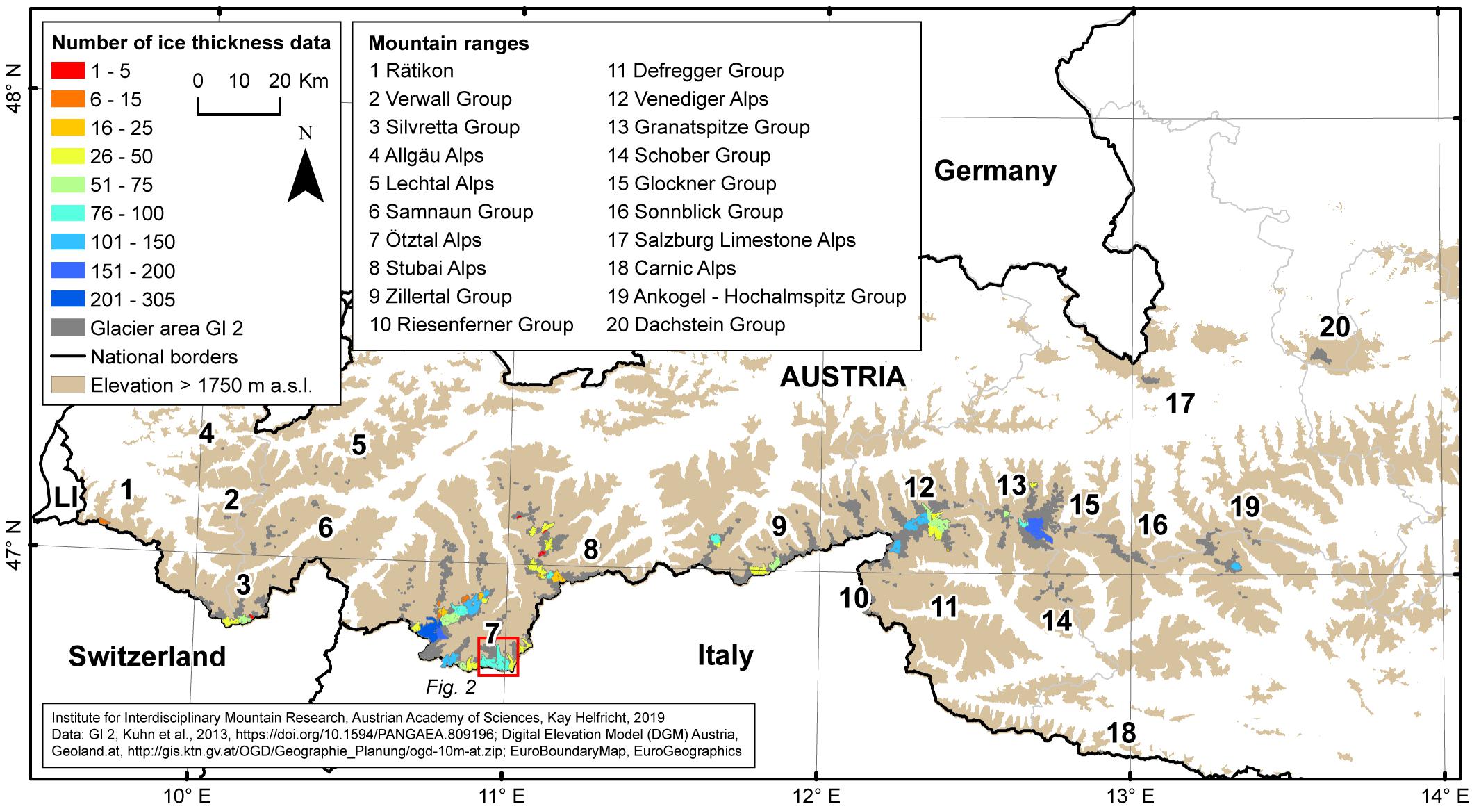
Figure 1. Location of the glaciers according to the second Austrian glacier inventory (gray area, GI 2) overlaid by all glaciers with available ice thickness measurements in color showing the number of ice thickness data points per glacier. The mountain ranges are indicated. The dashed red box highlights the zoom section presented in Figure 2. The brownish layer shows mountain areas with an elevation above 1750 m a.s.l.
Mass Balance Data
Continuous annual mass balance data exist from nine glaciers in Austria for the period between 2006 and 2016. Data are made available by the World Glacier Monitoring Service (WGMS, 2017 and former issues, http://wgms.ch/products_gmbb/, for Hintereisferner, Kesselwandferner, Pasterze, Sonnblickkees, Vernagtferner, Wurtenkees) and on PANGAEA data repository for Jamtalferner (Fischer et al., 2016a), Hallstätter Gletscher (Fischer et al., 2016b) and Mullwitzkees (Stocker-Waldhuber et al., 2016). More details on mass balance of the glaciers in Rofental valley (Hintereisferner, Kesselwandferner and Vernagtferner) are presented by Strasser et al. (2018) and for Mullwitzkees and Hallstätter Gletscher by Stocker-Waldhuber et al. (2013).
Materials and Methods
Ice Thickness Model
We used the approach of Huss and Farinotti (2012) for ice thickness modeling. The HF model was developed from the ice thickness estimation method presented by Farinotti et al. (2009b). The HF model scored highest among the automated methods applicable at large scales compared within the Ice Thickness Models Intercomparison Experiment (ITMIX, Farinotti et al., 2017) and has already been applied to all glaciers globally (Huss and Farinotti, 2012) and for regional glacier volume studies (e.g., Frey et al., 2014; Andreassen et al., 2015).
The basic principle of the HF model is the estimation of ice volume flux along the glacier, from which local ice thickness is computed based on measured surface slope and the flow law for ice. The approach accounts for basal sliding conditions, variations in the valley shape, and the influence of ice temperature on ice flow using several adjustable parameters. The surface mass balance and the volumetric balance flux are calculated along a simplified two-dimensional longitudinal profile of the glacier for estimating the mean ice thickness of individual elevation bands. In a final step, elevation band thicknesses are extrapolated to all cells of a regular grid depending on local surface slope and the distance from the glacier margin. We refer the reader to Huss and Farinotti (2012) for more details on the model architecture.
The H-model requires digitized glacier outlines and a DEM as input. We ran the model for 10 m elevation bands from glacier outlines and glacier surface elevations on the basis of DEMs with 10 m resolution from the three Austrian Glacier Inventories, GI 1 (1969), GI 2 (∼1998), and GI 3 (∼2006). Parameters on valley shape factor, continentality and climate were kept as proposed in Huss and Farinotti (2012).
Model Calibration
Homogenization of Ice Thickness Measurements to Glacier Inventory Dates
Temporal offsets between the ice thickness measurements and the surveys for the individual GIs exist. We have homogenized the ice thickness measurements of each glacier to the date of the GI 2 glacier surface with respect to the year of ice thickness measurements, which ranges from 1995 to 2010, and the date of GI 2 topographic survey, which ranges from 1996 to 2002. First, we calculated mean annual ice thickness changes between GI 2 and GI 3 from the change in observed surface elevation (z). The product of mean annual surface elevation changes and the number of years (y) between GI 2 and the date of ice thickness measurements was added to measured ice thickness (hM) for calculation of GI 2 ice thickness (hGI2).
The ice thickness (h) at the same location, but for the dates of GI 1 and GI 3, was calculated using the observed surface elevation changes between the respective glacier inventory and GI 2.
The uncertainty of the ice thickness (σIT) was computed based on error propagation accounting for thickness measurement uncertainty (7.5%), for the homogenization of ice thickness to GI 2 (1%), and for the DEM differencing to compute ice thickness changes between the inventory dates GI 2 and GI 1 (4%), as well as GI 2 and GI 3 (3%). The overall uncertainty of point thickness (11% for GI 1, 8% for GI 2, 13% for GI 3) is highest for GI 3 because of lower mean ice thickness.
Glacier-Specific Calibration of Apparent Mass Balance Gradient
The HF model requires an estimate of the apparent mass balance gradient to calculate ice volume flux along the glacier (Huss and Farinotti, 2012). The apparent mass balance () is defined as
where is the surface mass balance, ρ is the density of ice (i) and water (w), respectively, and ∂h/∂t the surface elevation change. In case of a balanced glacier mass budget and a glacier in steady-state, is equal to the surface mass balance and most negative at the glacier tongue and zero at the equilibrium line altitude (ELA). Surface ice melt is not totally compensated by ice flow in times of glacier retreat and increasingly imbalanced glacier states. Thus, surface elevation change converges toward surface mass balance and absolute values of will decrease, causing declining apparent mass balance gradients. The apparent mass balance gradient, varying for ablation and accumulation areas by a factor, which reduces the gradient for accumulation areas, is the primary parameter of the HF model in need of calibration as it varies between different regions and glacier types and is difficult to estimate without a priori information (Huss and Farinotti, 2012). We altered the apparent mass balance gradient for each of the 58 glaciers and each of the three GIs individually in an effort to minimize the mean absolute error (MAE) between modeled ice thickness (hmod) and the observed ice thickness data of the respective GI (hobs) for each individual glacier evaluated over all available point measurements (n):
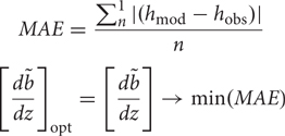
With our model setup we aim at reproducing average glacier thicknesses for calculating total ice volume. Thus, we also evaluate the mean error (ME) between all modeled and measured ice thickness of the individual glaciers with calibration data.
We applied cross-validation for estimating the model performance in reproducing single ice thickness measurements at the individual glaciers. Therefore, the available ice thickness data of each glacier have been randomly split into a calibration set and a validation set. The calibration set contained two thirds of the ice thickness data, and the validation set one third, respectively. For each glacier, this procedure has been repeated 150 times, allowing different, randomly chosen sets. The median of the MAE relative to the mean ice thickness of all 150 runs was calculated for the validation and calibration sets.
We also investigate whether the effect of increasingly imbalanced glacier states with decreasing difference between local surface mass balance and ice thickness change have to be considered by choosing an appropriate apparent mass balance gradient. Thus, we evaluate the difference in model performance by applying:
(i) calibrated glacier-specific apparent mass balance gradients,
(ii) calibrated apparent mass balance gradients averaged for the respective glacier inventory, and
(iii) the average apparent mass balance gradient derived in (ii) for GI 2 applied to all three GIs.
We compared the glacier-wide average of observed ice thickness change between the GIs with the difference in modeled ice thickness for the same inventories using all three options.
For estimating model performance for glacier-wide average ice thickness, we evaluated the average ME, its standard deviation and the average MAE, both in absolute values and relative to mean ice thickness, over all 58 glaciers applying calibration procedure (i). We tested two different methods of averaging calibrated mass balance gradients for transferring them to unmeasured glaciers, using overall mean optimal parameters and mean optimal parameters separated for the glacier size classes <1 km2, 1 – 5 km2, >5 km.
Calculation of Total Glacier Volume
For the calculation of total glacier volume we merged the ice thickness estimates of the 58 glaciers derived from glacier-specific calibration with the ice thickness calculations for all remaining glaciers applying the mean optimal d/dz for each glacier inventory and the three different size classes. Glacier volumes were analyzed for a subset of 775 glaciers, which are covered by glacier outlines and DEMs for all three GIs. In addition, we present a total volume including all glaciers of the inventories.
Recent Glacier Volume (2016)
To present a rough estimate of recent total glacier volume in Austria, we extrapolated the observed mass losses from nine representative glaciers with direct mass balance measurements to the overall glacier volume. We computed the total ice thickness change (Δh) from cumulated annual specific mass balances, considering the average area between GI 3 (about 2006) and the year 2016, and an estimated density of 900 kg m-3. The mean ice thickness change Δh so derived was compared to the mean ice thickness of all glaciers in GI 3 computing relative glacier volume changes since the last glacier inventory.
Results
Model Calibration and Validation
The overall average of all ice thickness point measurements is 72.6 ± 5.4 m and corresponds to a mean survey year of 2001. On average, acquisition of ice thickness measurements and the date of GI 2 were 3 years apart, with a mean ice thickness change of 4.0 ± 0.8 m. The mean ice thickness change calculated from surface elevation changes at the ice thickness measurement points between GI 1 and GI 2 is –11.2 ± 3.8 m in 29 years. The mean ice thickness change at the ice thickness measurement points between GI 2 and GI 3 is –11.3 ± 2.2 m within 10 years. Mean ice thickness at the measurement points is 88 ± 10.0 m, 76.7 ± 6.2 m, and 65.5 ± 8.4 m for GI 1, GI 2, and GI 3, respectively.
Figure 2 shows the available data and computed ice thickness distribution for Gurgler Ferner and some nearby glaciers as an example for all glaciers. The ice thicknesses modeled using the HF model not necessarily reproduced the measured point ice thicknesses everywhere, but modeled bedrock elevation along the flow line matches largely for all three GIs (Figure 2A).
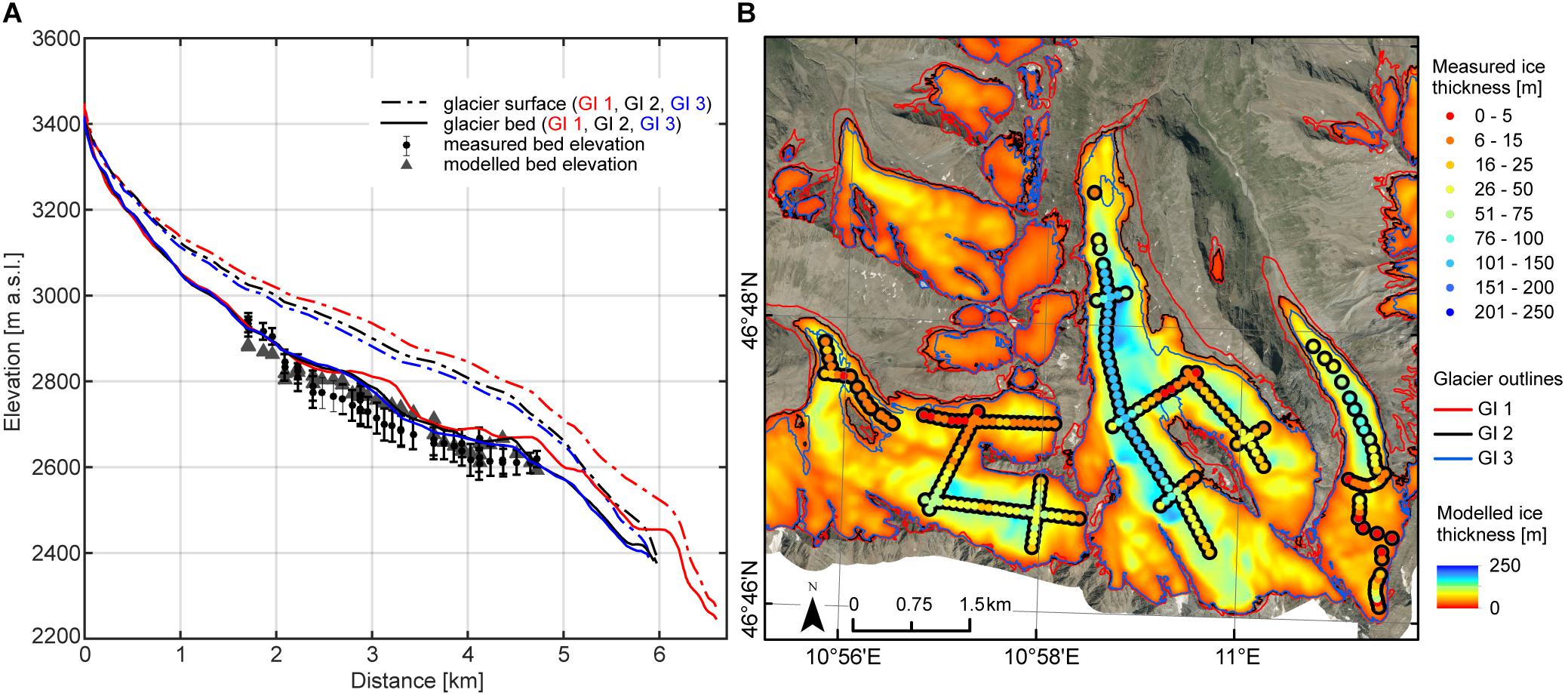
Figure 2. (A) Mean glacier surface elevation from 10 m – elevation bands for the respective glacier inventories GI 1 (red), GI 2 (black), and GI 3 (blue), and the glacier bed modeled using the HF model are shown with the measured and modeled bed elevation for locations of ice thickness measurements at Gurgler Ferner. The stems show the uncertainty of the ice thickness measurements. Measured and modelled ice thickness are presented in (B) highlighting the available data basis glacier outlines, the locations of ice thickness measurements and the modeled ice thickness distribution.
We found a high spread of optimal apparent mass balance gradients among the individual glaciers, a clear sign that we need ice thickness data for different glacier types to reasonably constrain the ice thickness model (Figure 3A). Apparent mass balance gradients decreased with a significant trend (p < 0.05) between GI 1 and GI 3, as well as for the sub-periods GI 1 to GI 2 and GI 2 to GI 3. The mean apparent mass balance gradient was reduced differently between the GI dates with respect to glacier size. It is reduced by 22% for small glaciers (<1 km2), by 33% for medium size glaciers (1–5 km2), and by 58% for larger glaciers from GI 1 to GI 3 (Table 1).
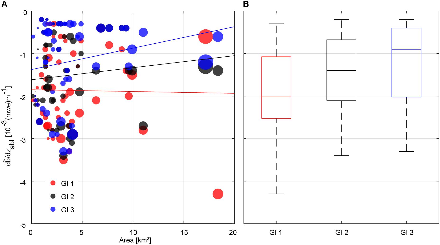
Figure 3. (A) Calibrated glacier-specific apparent mass balance gradients (d/dzabl) for the three glacier inventories. The size of the dots corresponds to the number of available ice thickness measurements. (B) The boxplots present the statistical distribution of the calibrated apparent mass balance gradients for the ablation area (d/dzabl) and the three glacier inventories. The blue box shows the interquartile range between the 25th and the 75th percentiles. The dash in the box notes the median. The whiskers encompass all data within 1.5 times the interquartile range.
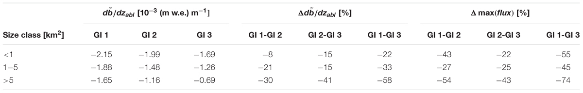
Table 1. /dzabl, its changes Δd/dzabl and changes of the maximum modeled flux Δmax(flux) between the glacier inventories (GI) separated for the three glacier size classes.
The applied cross-validation between modeled and measured point ice thickness at the individual glaciers results in MAE s relative to the observed ice thickness of 25–31% at the validation and calibration points (Table 2).
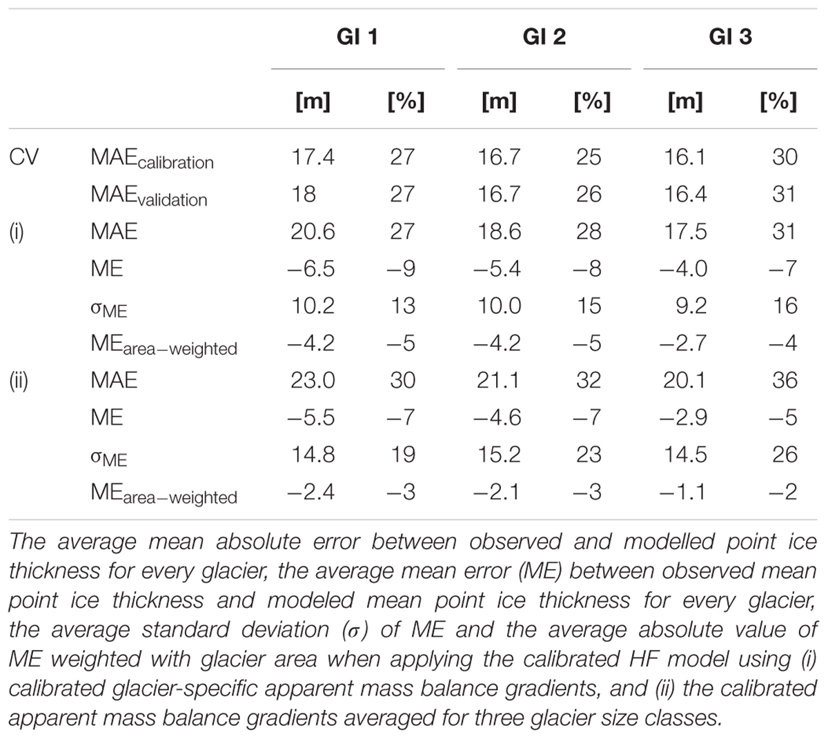
Table 2. Results of the cross-validation (CV) showing the median of the mean absolute error (MAE) from calibration and validation sets for all calibration glaciers from the three glacier inventories (GI).
HF-modeled ice thickness changes using option (i) and option (ii) resulted much closer to observed changes than using option (iii) for periods GI 1 to GI 2 (Figure 4) and GI 2 to GI 3. Ninety three percent of the observed mean ice thickness change could be reproduced using glacier-specific apparent mass balance gradients (Figure 4B). Eighty five percent of the observed mean ice thickness change was calculated using option (ii). Only 60% of the observed mean ice thickness change was modeled using option (iii).
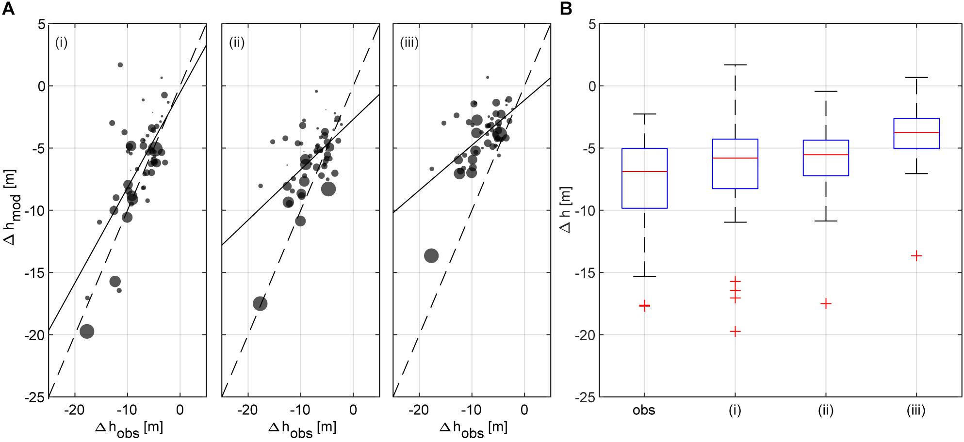
Figure 4. (A) Modeled versus observed glacier-wide mean ice thickness change between glacier inventories GI 1 and GI 2 using (i) calibrated glacier-specific apparent mass balance gradients, (ii) calibrated average apparent mass balance gradients for the respective glacier inventory, and (iii) a mean apparent mass balance gradient calibrated to GI 2 only. The boxplots in (B) present the statistical distribution of the glacier-wide mean thickness changes from observations between the glacier inventories (obs) and calculated from modeled ice thickness distributions with approaches (i) to (iii). The red dash notes the median, and the blue box shows the interquartile range between the 25th and the 75th percentiles. The whiskers encompass all data within 1.5 times the interquartile range. The red crosses present values that are more than 1.5 times the interquartile range away from the top or bottom of the box.
For selecting the parameters to be transferred to unmeasured glaciers we considered the area of glaciers without calibration data in comparison to the area of the calibration glaciers (Figure 5). We found that unmeasured glaciers make up for a very high fraction in the size class of less than 1 km2 (60% of total area), whereas calibration glaciers with an area of less than 1 km2 only have a share of 5%. Thus, we tested two different methods transferring calibrated apparent mass balance to unmeasured glaciers. Figure 6 shows the absolute error relative to glacier average ice thickness computed from measurements for optimal calibrated apparent mass balance gradients. In general, the absolute error is relatively high also for optimal model calibration at small glaciers. Particularly for glaciers smaller than 1 km2 and larger than 5 km2, the parameters separated for the three size classes show a distinct improvement in model performance in comparison to average parameters. This improvement is less significant for glaciers between 1 and 5 km2.
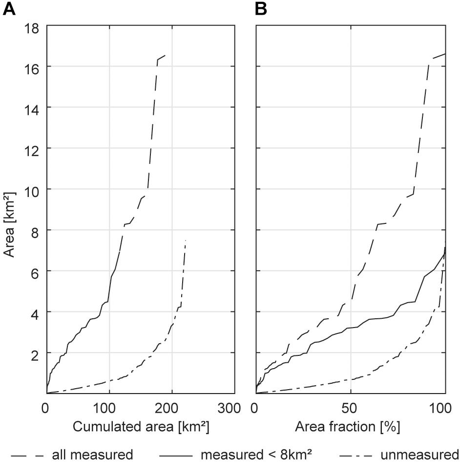
Figure 5. Cumulative glacier area distribution (A) in absolute numbers, and (B) relative to the total area for all glaciers with ice thickness measurements (dashed line), all glaciers with ice thickness measurements smaller than 8 km2 (solid line) and all glaciers without ice thickness measurements (dash-dotted line).
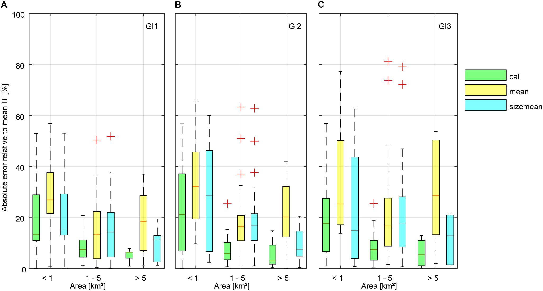
Figure 6. Absolute error between average glacier ice thickness from thickness measurements and modeled glacier mean ice thickness using the calibrated apparent mass balance gradients (cal), overall mean parameters (mean) and parameters for glacier size classes (sizemean) smaller 1 km2, 1–5 km2 and larger than 5 km2. Results are shown for all calibration glaciers of the three glacier inventories (A) GI 1, (B) GI 2, and (C) GI 3. The red dash notes the median, and the blue box shows the interquartile range between the 25th and the 75th percentiles. The whiskers encompass all data within 1.5 times the interquartile range. The red crosses present values that are more than 1.5 times the interquartile range away from the top or bottom of the box.
Model performance is presented both as absolute and relative values in Table 2 for the cross-validation, for glacier-specific calibration [option (i)], and for calibration to size classes mass balance [option (ii)]. The MAEs between the cross-validation and glacier-specific calibration are similar. For using average parameters, the MAE increases. While there is no great difference in MEs, the standard deviation and the absolute values of ME are higher when applying the bulk parameters, compared to the glacier-specific calibration.
Total Glacier Volume and Volume Changes
We used the mean optimal gradients derived for three different glacier area classes from the calibrated glacier-specific parameters to model the remaining ice volumes of glaciers without ice thickness measurements. Seven hundred and seventy five glaciers are covered by all three GIs (Table 3). The total volume of these glaciers decreased from 22.2 km3 for GI 1 to 15.6 km3 for GI 3. This means a volume loss of 30% between 1969 and 2006, while the total area decreased by 26%. The total volume for all glaciers in GI 3 is 15.9 km3.
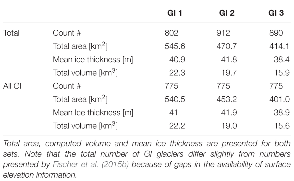
Table 3. Number of investigated glaciers for the total glacier inventory and for all glaciers with outlines covered by all GIs.
Glaciers larger than 1 km2 cover more than 65% of the total area and hold about 80% of the total volume (Figure 7), highlighting the importance of the large glaciers for overall volume. The 10 largest glaciers with areas larger than 5 km2 make up more than 20% of the total area and nearly about 35% of total volume for GI 3. Fifteen percent of the modeled total volume in the Austrian Alps is made up by the two largest glaciers, Pasterze and Gepatschferner.
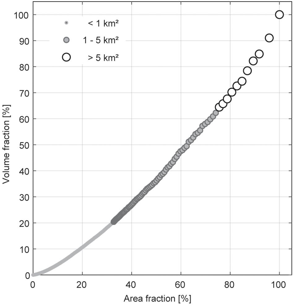
Figure 7. Cumulative volume fraction of the total glacier volume for all glaciers of GI 3 sorted by glacier area, also presented as cumulative area fraction. Note that dots are scaled and shaded by the glacier area classes smaller than 1 km2, 1–5 km2, and larger than 5 km2.
As regards changes in area and volume between the GIs for different glacier sizes, the largest absolute changes occur for largest glaciers (Figure 8A). Glaciers smaller than 1 km2 lost 40% of their area and more than 50% of their volume (Figure 8B), and contributed by 1.9 km3 to the total volume loss of 6.6 km3 between GI 1 and GI 3 (Figure 8A). The total volume loss of glaciers between 1 and 5 km2 was 2.4 km3, and 2.2 km3 for glaciers larger than 5 km2, respectively. In general, relative changes in area and volume were larger for small glaciers compared to glaciers larger than 1 km2, and relative volume changes are higher than relative area changes for all considered time periods (Figure 8B).
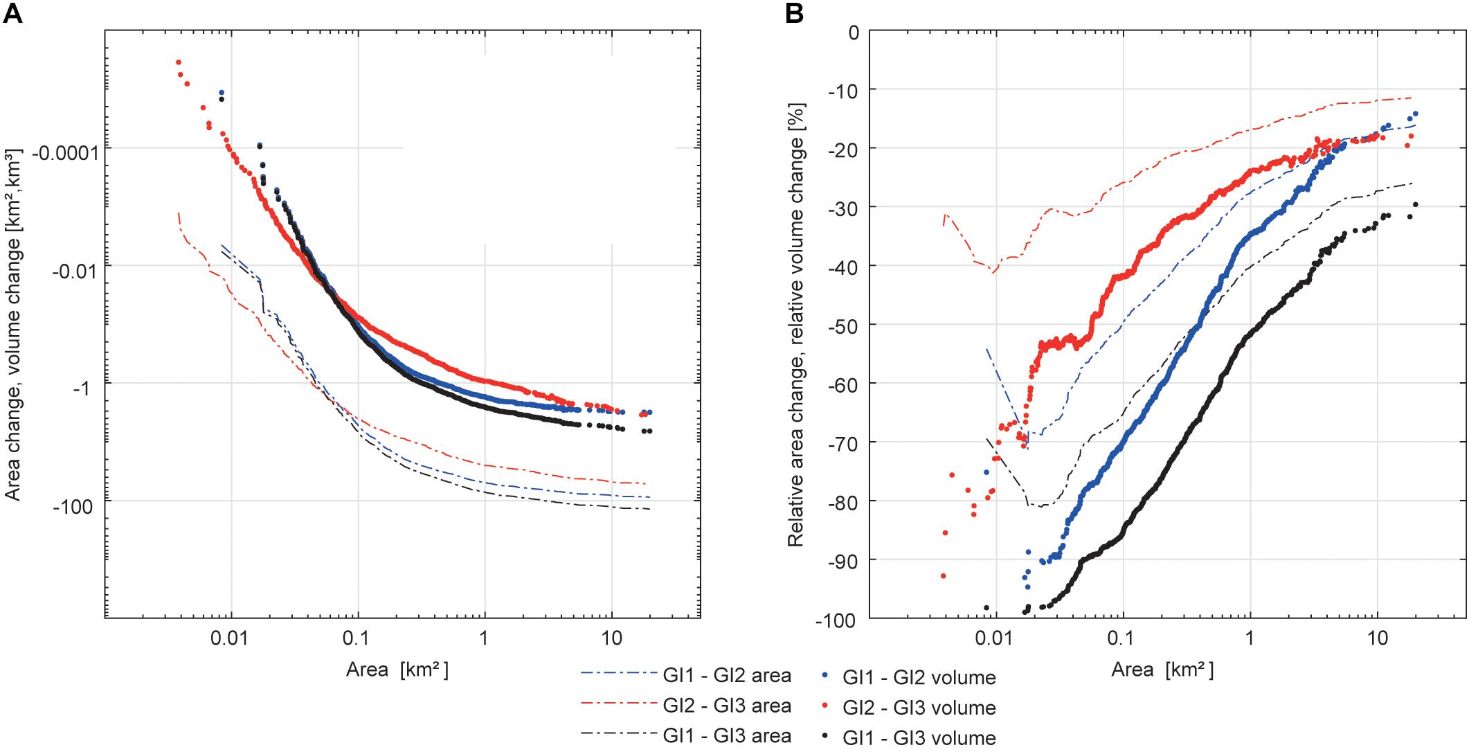
Figure 8. (A) Cumulative absolute changes in area and volume and (B) cumulative changes of area and volume relative to glacier area and glacier volume between the glacier inventories (GI) for all glaciers sorted by glacier area. Note the logarithmic scale for the glacier area and absolute change values.
This is also valid separated for different mountain regions in Austria (Figure 9). Relative changes in area and volume are smaller in regions with many and large glaciers, e.g., Glockner Group, Ötztal Group, Stubai and Venediger Group. Highest relative volume changes were modeled for the very small to medium-sized glaciers along the northern fringe of the Alps, such as in the Rätikon and the Salzburger Limestone Alps, for the period GI 1 to GI 2, but also in the Allgäu Alps between GI 2 and GI 3. Here the glaciers have lower maximum altitudes than those at the main Alpine ridge. An exception is the Dachstein region with smaller changes than the glacier regions at the Alpine main ridge and south of it (e.g., Granatspitz Group, Schober Group).
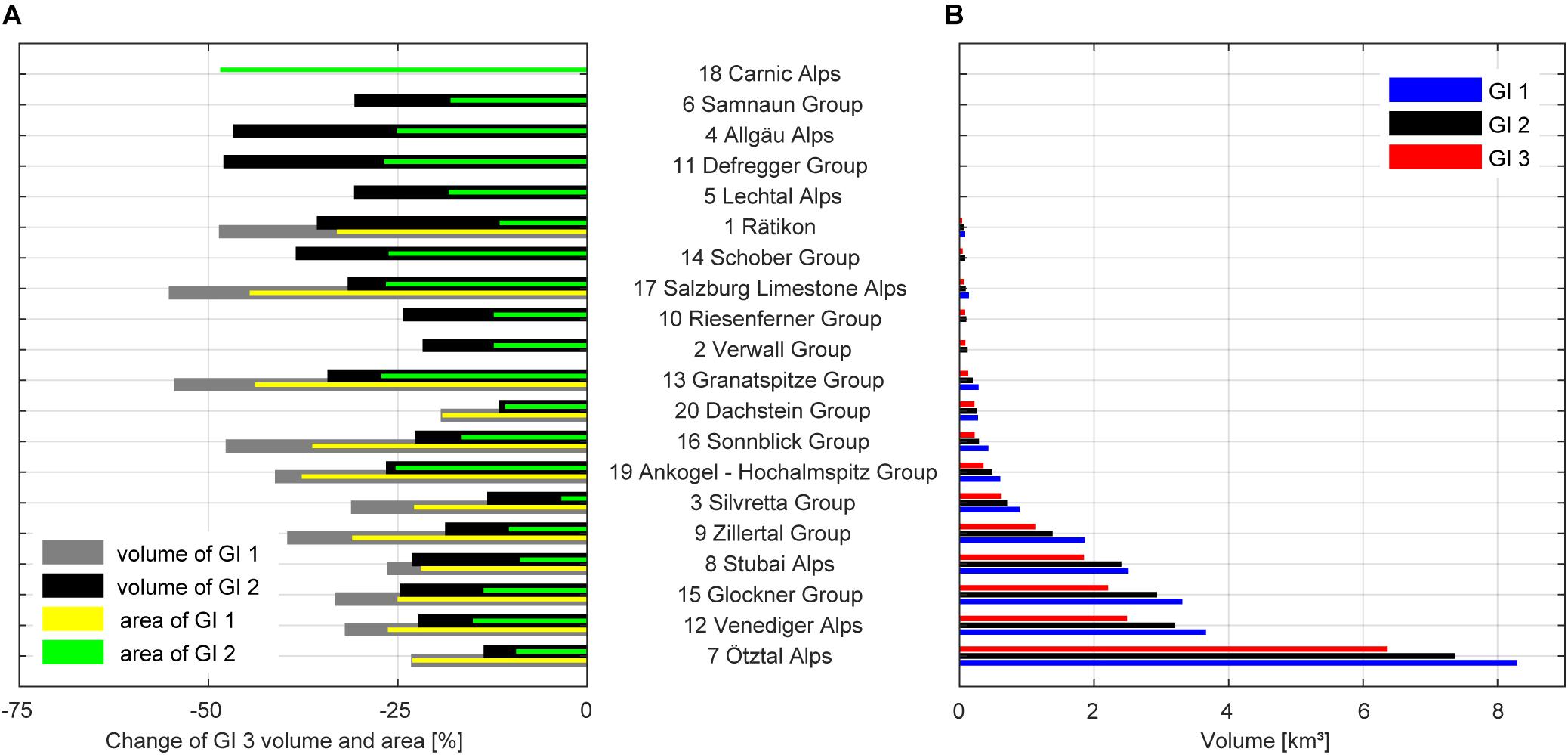
Figure 9. (A) Relative changes in volume and area from GI 1 and GI 2 to the latest glacier inventory (GI 3) and (B) total volume of all glaciers in the respective mountain ranges. The five smallest volumes are less than 0.01 km3. Regions are ordered according to increasing total ice volume.
Recent Glacier Volume (2016)
Mean measured specific mass balances (b) from nine glaciers in Austria of the period between GI 3 and 2016 are presented in Table 4. The overall mean annual mass balance for this period is -949 ± 100 mm, which corresponds to a mean ice thickness change of -1.1 ± 0.1 m per year and -8.4 ± 0.9 m between GI 3 and 2016. This is 22 ± 2.3% of the GI 3 mean ice thickness and equals a volume change of -3.5 ± 0.4 km3. Thus, the estimate for recent total glacier volume (2016) is 12.4 km3.
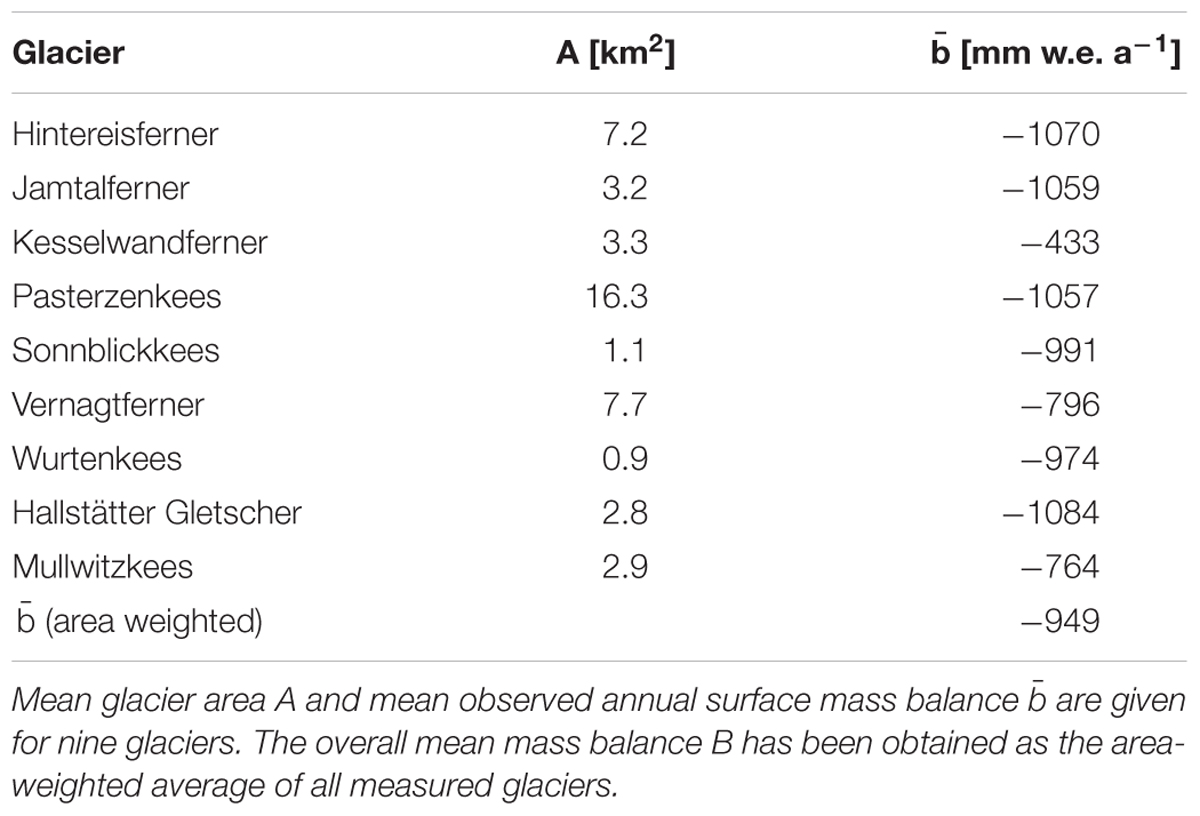
Table 4. Observed average glacier mass balances between GI 3 and 2016.
Discussion
The present study uses a set of data of varying quality and uncertainties. Ice thickness measurements have been performed over a period of 15 years, applying different spacing of measurements, different antenna frequencies and different spatial coverage of the respective glaciers (Span et al., 2005; Fischer et al., 2007, 2015c). The uncertainty of the DEMs was considered when estimating the uncertainty in ice thickness of different glacier inventory dates. From a modeling perspective, the ITMIX experiment (Farinotti et al., 2017) concluded that mean deviations of modeled ice thickness from direct ice thickness measurements are in the order of 10%, whereas the standard deviation between individual models resulted in 24%. Taking all sources of error related to ice thickness measurements, surface elevation surveys and ice thickness modeling into account, relative uncertainties can easily aggregate to 30% (e.g., Huss and Farinotti, 2012).
We performed a cross-validation between modeled and measured point ice thickness, which indicates model errors of 25–31% (Table 2). The MAE averaged for all calibrated glaciers is similar for the calibration using option (i), and increases to 30–36% using option (ii). These errors refer to the overall uncertainty in the ice thickness and volume calculations. However, for reproducing glacier average characteristics, the model bias can be interpreted in terms of model performance for calculating the total glacier ice volume (e.g., Farinotti et al., 2017). We find a negative bias in the glacier-wide average of modeled point ice thickness in comparison to the observations indicating that overall ice volume might be slightly underestimated by our approach. Applying an area-weighting of the bias results in an average mean bias in mean ice thickness of -5% for glacier-specific calibration and -3% for global parameters (Table 2). This small difference would imply better average results for option (ii), but the MAEs and the standard deviation of the bias are lower for option (i) compared to option (ii). This highlights the great value of ice thickness information for capturing the high variability in mean glacier ice thickness, which is not strictly related to glacier area.
Although distributed thickness measurements are provided, the presented calibration aims at reproducing mean characteristics, and not individual measurements. Additional parameters controlling ice thickness, such as surface slope and glacier width, are not incorporated in scaling relationships, but are considered in flux-based models such as the HF method. We have tested an alternative version of the HF2012-model that is capable of assimilating individual ice thickness measurements to 58 glaciers with direct observations. The experiment showed that the resulting ice thickness distribution did not importantly change, and the overall ice volume estimates remain almost unaffected. The volume of glaciers with calibration differed by 2%, with a mean absolute difference of 10% to modeled volume presented in this study. Computationally more expensive approaches (e.g., Morlighem et al., 2011; Fürst et al., 2017) are well capable of assimilating direct measurements. As our goal is to apply a calibrated model to all glaciers in Austria, most of which are not covered by direct observations, we preferred to stay with the simple forward method.
We found that ice thickness at very small glaciers (<1 km2) cannot be satisfactorily simulated with the applied model. This suggests that ice thickness modeling based on glacier inventory data is still too uncertain to independently infer glacier volume changes of individual small glaciers. This is partly due to the observed high spatial variability in geodetic mass balance, even of neighboring glaciers (Abermann et al., 2010; Fischer et al., 2015d), which also may be caused by heterogeneity in snow deposition caused by avalanche activity or wind drift, and other factors such as different response times. In general, the transferability of the calibrated apparent mass balance gradients to other mountain regions appears to be problematic. From the calibration we found no significant relation between apparent mass balance gradients and area or slope of the glaciers with ice thickness measurements. Further, the apparent mass balance appeared to change between the dates of the GIs with respect to the actual glacier states. Thus, more than topographic conditions, the balance or imbalance of the modeled glaciers has to be considered for estimating model parameters. This study shows that ice thickness changes for a sample of about 50 glaciers can be simulated with reasonable accuracy (Figure 4). However, the calibration of the model revealed the necessity to adapt parameters controlling mass flux in the ice thickness model to the glacier states at a specific point in time.
Farinotti et al. (2009b) found an optimized apparent mass balance gradient of -0.0055 (m w.e.) m-1 for four glaciers in the Swiss Alps. This is considerably higher than the values we found for glaciers in Austria (Table 1). However, this may be caused by the difference in glacier size and ice flow velocities of the glaciers in Austria compared to the glacier systems like considered by Farinotti et al. (2009a).
The total volume estimate presented in this study is higher than that of Patzelt (1978) for GI 1 (21 km3), and surpass the estimates by Lambrecht and Kuhn (2007) for GI 2 (17.7 km3) derived from volume-area scaling by 11%. Applying the volume-area scaling relation used by Lambrecht and Kuhn (2007) to all GI 3 glaciers results in a total volume of 14.9 km3, which is again 7% lower than our computed overall volumes. Although the overall results do not differ substantially, the present study also allows specifying volumes, thickness distribution and bedrock maps for individual glaciers, which will be a considerable benefit for climate change impact studies. Nevertheless, changes in glacier states and glacier geometries (e.g., change in hypsometry) can be assumed to be not covered using simple scaling relationships.
Farinotti et al. (2019) used an ensemble of up to five models to provide a consensus estimate for the ice thickness distribution of all glaciers outside the Greenland and Antarctic ice sheets, and thus also for Austrian glaciers. Their estimate is based on glacier outlines of the Randolph Glacier Inventory (RGI) 6.0 (RGI Consortium, 2017) and the surface topography from the Shuttle radar topography mission (SRTM) DEM version 4 (Jarvis et al., 2008). The glacier outlines in the RGI are digitized automatically from landsat thematic mapper (TM) data and differ in date and, a little, in shape from the Austrian glacier inventories. The surface topography from SRTM is based on satellite data from around the year 2000. The results of Farinotti et al. (2019) cover a set of 742 glaciers in Austria, with a total area of 365.9 km2. Their composite estimate of the total ice volume is 18.9 km3, which corresponds to a mean ice thickness of 51.6 m.
In general their consensus estimate for the total glacier volume in Austria is similar to the GI 2 estimate presented in this study. This corresponds to the earlier data basis used by Farinotti et al. (2019), which is close to the dates of GI 2. However, their mean ice thickness estimate is 10 m higher than the ice thickness estimate presented here. This may be a result of the composite ice volume on the results of the individual models by Farinotti et al. (2019), but also by generally assuming higher mass turnover for the individual glaciers and thus a fairly balanced glacier state. In contrast, the lower mean ice thickness presented here is a result of the reduction of the apparent mass balance gradient as presented in the calibration.
The big relative change in area and volume of very small glaciers (<0.5 km2) found in the model results (Figure 8) was also made evident by Lambrecht and Kuhn (2007) between GI 1 and GI 2, by Abermann et al. (2009) particularly for the Ötztal mountain range and by Fischer et al. (2014) for small glaciers in the Swiss Alps. Further, ice thickness measurements particularly at small glaciers show, that their ice thickness and volume are often underestimated by model estimations. In this study we focused on the transfer of individual parameters considering glacier size, which, caused by the high number of small glaciers, increases the modeled ice volume also compared to former applications of the HF model by some percent.
Our calibration set-up revealed that a reduction of ice flux over the last five decades can be directly detected by constraining the ice thickness model with multi-temporal glacier inventory data and ice thickness observations. Decreasing ice fluxes are also supported independently by ice velocity measurements. The vertical surface velocity has been measured at stake locations on Kesselwandferner (Ötztal Alps) since the 1960s. Stocker-Waldhuber et al. (unpublished) presented an analysis of this exceptional data set, showing the substantial reduction, both in the horizontal and the vertical component of ice flow, at the end of the 1980s. On average, ice flux was reduced by a factor of 3 at the ELA over a period of approximately 10 years. This is in line with the changes in apparent mass balance gradients and maximum ice flux as derived from the model calibration (Table 1). Between GI 1 and GI 3, the maximum ice flux modeled along the glacier (i.e., ice flux at the apparent equilibrium line) was reduced by two thirds applying the calibrated parameters for large glaciers (>5 km2). Even for very small glaciers, the reduction in mass flux was found to be 35%, which is, however, mainly related to changes in glacier area rather than changes in the calibrated apparent mass balance gradients for this glacier size class.
In times of a simultaneous availability of both direct glaciological and geodetical glacier mass balances (e.g., Thibert et al., 2008; Huss et al., 2009; Klug et al., 2018), the apparent mass balance as the difference between both, and thus the actual state of the glaciers, can be estimated. We applied a simple direct determination of apparent mass balance gradients using data of the glaciological and geodetical mass balance in 100 m elevation bands to Hintereisferner, Kesselwandferner and Vernagtferner for the periods between the three GIs (Table 5). Although this rough calculation includes several sources of uncertainty, the trend of decreasing apparent mass balance gradients is clear, as for our optimal model parameters (Figure 3B), with a substantial reduction in the most recent period. However, we also stress that a direct comparability between our optimized model parameters, constrained for matching the ice thickness observations, and the apparent mass balance gradients inferred from field data is difficult for the following reasons: (i) Uncertainties in in situ mass balances are considerable, (ii) the gradients are often not linear in reality which complicates the computation of apparent mass balance gradients (theoretical concept), (iii) the numbers refer to decadal/multi-decadal periods instead of single points in time as for the optimal model parameters. Considering the glacier advance in the 1980s followed by a strong and accelerating retreat since the 1990s, the large difference between the observations may be explained by imbalanced glacier states with extreme ratios between surface mass balance and surface elevation changes. In the model, however, GI 1 marks the time before glacier advance, at time of GI 2 glaciers already started to lose mass, and ice flux has been strongly reduced toward GI 3. This indicates that absolute values are difficult to compare but the order of magnitude of the inferred apparent mass balance gradients, as well as the general trend toward a decrease over time is revealed in both the field data and the calibrated model parameters.
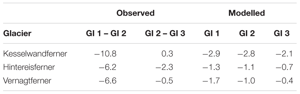
Table 5. Apparent mass balance gradients d/dzabl in 10-3 m w.e. m-1 for the ablation zones of the three glaciers calculated as difference from specific mass balance data of 100 m elevation bands originating from glaciological measurements and geodetically derived mass balance from DEM differencing between the dates of GI 1 to GI 2 and GI 2 to GI 3.
The high variability of volume loss in the specific regions in the different periods means that, despite an undoubted general climate signal, the individual timing and course of the response of the glaciers needs a high model resolution when regional changes at decadal time scales are to be tackled. The course of thinning, decrease of dynamics and a final area loss is not only influenced by climate, but also by topography and small-scale local climate variabilities. Our study reveals that the rate of area loss is not similar to the rate of volume loss, but varies from glacier to glacier, region to region and with glacier size.
Conclusion
In the present study, we applied an extensive calibration scheme for estimating the ice volume of all glaciers in Austria. We investigated temporal changes of the apparent mass balance and controlled the glacier mass turnover within the utilized ice thickness model. A comprehensive data set of in-situ ice thickness measurements at 58 glaciers and data on glacier surface elevation and extent from three GIs between 1969 and 2006 was used. We found that calibrated apparent mass balance gradients differ considerably between the GIs, with a significant trend toward a reduction in the gradients. This demonstrates the increasingly unbalanced conditions of glaciers in the Austrian Alps due to a considerable reduction of ice flow, which is not only presented in the calibration of the apparent mass balance, but also manifested in comparison of geodetic and glaciological mass balances and in observations over the last decades. The observed ice thickness changes between the three inventories could be simulated with acceptable accuracy using the calibrated glacier-specific apparent mass balance gradients and averaged calibrated gradients of the respective GIs, but results were more uncertain when fixed parameters for all three GIs were used. Changing glacier dynamics of Alpine glaciers in recent decades significantly affect the modeling of distributed mountain glacier volumes and have to be incorporated in model design for ice thickness estimates.
We used the calibrated model for a volume estimation of all glaciers in Austria. The volume for the most recent Austrian glacier inventory (GI 3, around 2006) is 15.9 km3. This would be enough to cover Austria’s entire territory with 0.19 m of water. Updated to 2016, we estimate an ice volume of 12.4 km3, indicating an overall loss of 22% of the Austrian glacier volume only over the last decade.
Our study highlights the imbalance between the number of glaciers, glacier area and volume. A high number of very small glaciers only make up a small part of the total ice volume, while a few large glaciers store much of the total ice volume. This also affects the present and future change rates of glacier area and glacier volume in Austria. In general, relative volume changes are higher than relative area changes up to GI 3. However, with ongoing thinning of the glaciers this relation could be expected to change toward higher rates of area loss. The high variability of loss rates between specific types and regions means that sophisticated monitoring strategies are still essential if needed as the basis for adaption strategies to climate change.
We demonstrate the importance of ice thickness measurements for correctly estimating glacier ice volume with respect to actual glacier states. This is particularly important for improving ice thickness estimates for Alpine glaciers that are close to significant shifts in glacier dynamics, like Austria’s largest glaciers. Our new estimates of glacier mean ice thickness form the basis for various impact studies from local to regional level regarding future glacier retreat, natural hazards and changes in mountain hydrology.
Author Contributions
KH designed the study, performed all calculations, produced all figures, and wrote the manuscript together with MH. MH. provided the model code and processed all input data. MH, AF, and J-CO contributed significantly to the study framework and the discussion of the results.
Funding
The FutureLakes project (Formation and future evolution of glacier lakes in Austria) was funded by the Earth System Sciences Call (ESS), an initiative of the Austrian Academy of Sciences (ÖAW). Project duration 03/2015 – 02/2018 (Helfricht et al., 2019a,b).
Conflict of Interest Statement
The authors declare that the research was conducted in the absence of any commercial or financial relationships that could be construed as a potential conflict of interest.
Acknowledgments
We would like to thank Michael Kuhn for the discussion of the Austrian glacier inventories and for providing data. We would like to thank the regional authorities for providing digital elevation models for the generation of the third Austrian glacier inventory. We gratefully acknowledge Brigitte Scott for the professional English editing, and all researchers collaborating within the FutureLakes team. And we would also like to thank the two reviewers for the constructive feedback. Their comments contributed greatly to the manuscript.
References
Abermann, J., Fischer, A., Lambrecht, A., and Geist, T. (2010). On the potential of very high-resolution repeat DEMs in glacial and periglacial environments. Cryosphere 4, 53–65. doi: 10.5194/tc-4-53-2010
Abermann, J., Lambrecht, A., Fischer, A., and Kuhn, M. (2009). Quantifying changes and trends in glacier area and volume in the Austrian Ötztal Alps (1969-1997-2006). Cryosphere 3, 205–215. doi: 10.5194/tc-3-205-2009
Andreassen, L., Huss, M., Melvold, K., Elvehøy, H., and Winsvold, S. (2015). Ice thickness measurements and volume estimates for glaciers in Norway. J. Glaciol. 61, 763–775. doi: 10.3189/2015JoG14J161
APCC. (2014). Österreichischer Sachstandsbericht Klimawandel 2014. Austrian Panel on Climate Change (APCC). Wien: Verlag der Österreichischen Akademie der Wissenschaften.
Auer, I., Böhm, R., Jurkovic, A., Lipa, W., Orlik, A., Potzmann, R., et al. (2007). HISTALP—historical instrumental climatological surface time series of the Greater alpine region. Int. J. Climatol. 27, 17–46. doi: 10.1002/joc.1377
Bahr, D. B., Meier, M. F., and Peckham, S. D. (1997). The physical basis of glacier volume-area scaling. J. Geophys. Res. 102, 355–320. doi: 10.1029/97JB01696
Bahr, D. B., Pfeffer, W. T., and Kaser, G. (2015). A review of volume-area scaling of glaciers. Rev. Geophys. 53, 95–140. doi: 10.1002/2014RG000470
Buckel, J., Otto, J. C., Prasicek, G., and Keuschnig, M. (2018). Glacial Lakes in Austria - Distribution and Formation Since the Little Ice Age. Amsterdam: Global and Planetary Change.
Clarke, G. K. C., Berthier, E., Schoof, C. G., and Jarosch, A. H. (2009). Neural networks applied to estimating subglacial topography and glacier volume. J. Climate 22, 2146–2160. doi: 10.1175/2008JCLI2572.1
Colonia, D., Torres, J., Haeberli, W., Schauwecker, S., Braendle, E., Giraldez, C., et al. (2017). Compiling an inventory of glacier-bed overdeepenings and potential new lakes in de-glaciating areas of the peruvian andes: approach, first results, and perspectives for adaptation to climate change. Water 9:336. doi: 10.3390/w9050336
Emmer, A., Klimeš, J., Mergili, M., Vilímek, V., and Cochachin, A. (2016). 882 lakes of the cordillera blanca: an inventory, classification, evolution and assessment of susceptibility to outburst floods. Catena 147, 269–279. doi: 10.1016/j.catena.2016.07.032
Farinotti, D., Brinkerhoff, D. J., Clarke, G. K. C., Fürst, J. J., Frey, H., Gantayat, P., et al. (2017). How accurate are estimates of glacier ice thickness? results from ITMIX, the ice thickness models intercomparison eXperiment. Cryosphere 11, 949–970. doi: 10.5194/tc-11-949-2017
Farinotti, D., Huss, M., Bauder, A., and Funk, M. (2009a). An estimate of the glacier ice volume in the Swiss Alps. Glob. Planet. Chang. 68, 225–231. doi: 10.1016/j.gloplacha.2009.05.004
Farinotti, D., Huss, M., Bauder, A., Funk, M., and Truffer, M. (2009b). A method for estimating the ice volume and ice thickness distribution of alpine glaciers. J. Glaciol. 55, 422–430. doi: 10.3189/002214309788816759
Farinotti, D., Huss, M., Fürst, J. J., Landmann, J., Machguth, H., Maussion, F., et al. (2019). A consensus estimate for the ice thickness distribution of all glaciers on Earth. Nat. Geosci. 12, 168–173. doi: 10.1038/s41561-019-0300-3
Fischer, A., and Kuhn, M. (2013). Ground-penetrating radar measurements of 64 Austrian glaciers between 1995 and 2010. Ann. Glaciol. 54, 179–188. doi: 10.3189/2013AoG64A108
Fischer, A., Markl, G., and Kuhn, M. (2016a). Glacier Mass Balances and Elevation Zones of Jamtalferner, Silvretta, Austria, 1988/1989 to 2016/2017. Innsbruck. PANGAEA: Institute for Interdisciplinary Mountain Research Austrian Academy of Sciences.
Fischer, A., Stocker-Waldhuber, M., Reingruber, K., and Helfricht, K. (2016b). Glacier Mass Balances and Elevation Zones of Hallstätter Gletscher, Dachstein, Austria, 2006/2007 to 2016/2017. Innsbruck. PANGAEA: Institute for Interdisciplinary Mountain Research Austrian Academy of Sciences.
Fischer, A., Seiser, B., Stocker-Waldhuber, M., Mitterer, C., and Abermann, J. (2015a). The Austrian Glacier Inventories GI 1 (1969), GI 2 (1998), GI 3 (2006), and GI LIA in ArcGIS (shapefile) Format. Innsbruck. PANGAEA: Institute for Interdisciplinary Mountain Research Austrian Academy of Sciences.
Fischer, A., Seiser, B., Stocker Waldhuber, M., Mitterer, C., and Abermann, J. (2015b). Tracing glacier changes in Austria from the little ice age to the present using a lidar-based high-resolution glacier inventory in Austria. Cryosphere 9, 753–766. doi: 10.5194/tc-9-753-2015
Fischer, A., Span, N., Kuhn, M., Helfricht, K., Stocker-Waldhuber, M., Seiser, B., et al. (2015c). Ground-Penetrating Radar (GPR) Point Measurements of Ice Thickness in Austria. Innsbruck. PANGAEA: Institute for Interdisciplinary Mountain Research Austrian Academy of Sciences.
Fischer, M., Huss, M., and Hoelzle, M. (2015d). Surface elevation and mass changes of all Swiss glaciers 1980–2010. Cryosphere 9, 525–540. doi: 10.5194/tc-9-525-2015
Fischer, A., Span, N., Fischer, A., Kuhn, M., Massimo, M., and Butschek, M. (2007). Radarmessungen der Eisdicke Österreichischer Gletscher. Band II: Messungen 1999 bis 2006. Wien: Österreichische Beiträge zu Meteorologieund Geophysik.
Fischer, M., Huss, M., Barboux, C., and Hoelzle, M. (2014). The new swiss glacier inventory sgi2010: relevance of using high-resolution source data in areas dominated by very small glaciers. Arct. Antarct. Alp. Res. 46, 933–945. doi: 10.1657/1938-4246-46.4.933
Frey, H., Machguth, H., Huss, M., Huggel, C., Bajracharya, S., Bolch, T., et al. (2014). Estimating the volume of glaciers in the Himalayan–Karakoram region using different methods. Cryosphere 8, 2313–2333. doi: 10.5194/tc-8-2313-2014
Fürst, J. J., Gillet-Chaulet, F., Benham, T. J., Dowdeswell, J. A., Grabiec, M., Navarro, F., et al. (2017). Application of a two-step approach for mapping ice thickness to various glacier types on Svalbard. Cryosphere 11, 2003–2032. doi: 10.5194/tc-11-2003-2017
Gross, G. (1987). Der Flächenverlust der Gletscher in Österreich 1850-1920-1969. Zeitschrift für Gletscherkunde und Glazialgeologie 23, 131–141.
Gudmundsson, G. H. (1999). A three-dimensional numerical model of the confluence area of Unteraargletscher, Bernese Alps, Switzerland. J. Glaciol. 45, 219–230. doi: 10.1017/S0022143000001726
Haeberli, W., Buetler, M., Huggel, C., Lehmann, T., Schaub, Y., and Schleiss, A. J. (2016). New lakes in deglaciating high-mountain regions – opportunities and risks. Clim. Chang. 139, 201–214. doi: 10.1007/s10584-016-1771-5
Haeberli, W., and Linsbauer, A. (2013). Global glacier volumes and sea level – small but systematic effects of ice below the surface of the ocean and of new local lakes on land. Brief communication. Cryosphere 7, 817–821. doi: 10.5194/tc-7-817-2013
Haeberli, W., Whiteman, C., and Shroder, J. F. (eds) (2014). Snow and Ice-Related Hazards, Risks, and Disasters. Amsterdam: Elsevier.
Helfricht, K., Huss, M., Fischer, A., and Otto, J.-C. (2019a). Calibrated estimates of mean and maximum ice thickness for glaciers of the third Austrian Glacier Inventory (GI3). PANGAEA. doi: 10.1594/PANGAEA.898642
Helfricht, K., Huss, M., Fischer, A., and Otto, J.-C. (2019b). Spatial ice thickness distribution and glacier bed elevation for glaciers of the third Austrian Glacier Inventory (GI3). PANGAEA. doi: 10.1594/PANGAEA.898651
Hock, R., Hutchings, J. K., and Lehning, M. (2017). Grand Challenges in cryospheric sciences: toward better predictability of glaciers, snow and sea ice. Front. Earth Sci. 5:64. doi: 10.3389/feart.2017.00064
Huss, M., Bauder, A., and Funk, M. (2009). Homogenization of long-term mass-balance time series. Ann. Glaciol. 50, 198–206. doi: 10.3189/172756409787769627
Huss, M., and Farinotti, D. (2012). Distributed ice thickness and volume of all glaciers around the globe. J. Geophys. Res. 117:F04010. doi: 10.1029/2012JF002523
Huss, M., and Hock, R. (2015). A new model for global glacier change and sea-level rise. Front. Earth Sci. 3:54. doi: 10.3389/feart.2015.00054
Huss, M., and Hock, R. (2018). Global-scale hydrological response to future glacier mass loss. Nat. Clim. Chang. 8, 135–140. doi: 10.1038/s41558-017-0049-x
IPCC. (2014). in Climate Change 2014: Synthesis Report. Contribution of Working Groups I, II and III to the Fifth Assessment Report of the Intergovernmental Panel on Climate Change, eds R. K. Pachauri and L. A. Meyer (Geneva: IPCC).
Jarvis, A., Reuter, H. I., Nelson, A., and Guevara, E. (2008). Hole-filled SRTM for the Globe Version 4. Berlin: CGIAR Consortium for Spatial Information.
Kaser, G., Großhauser, M., and Marzeion, B. (2010). Contribution potential of glaciers to water availability in different climate regimes. Proc. Natl Acad. Sci. U.S.A. 107, 20223–20227. doi: 10.1073/pnas.1008162107
Klug, C., Bollmann, E., Galos, S. P., Nicholson, L., Prinz, R., Rieg, L., et al. (2018). Geodetic reanalysis of annual glaciological mass balances (2001–2011) of Hintereisferner, austria. Cryosphere 12, 833–849. doi: 10.5194/tc-12-833-2018
Lambrecht, A., and Kuhn, M. (2007). Glacier changes in the Austrian Alps during the last three decades, derived from the new Austrian glacier inventory. Ann. Glaciol. 46, 177–184. doi: 10.3189/172756407782871341
Li, H., Ng, F., Li, Z., Qin, D., and Cheng, G. (2012). An extended “perfect-plasticity” method for estimating ice thickness along the flow line of mountain glaciers. J. Geophys. Res. 117:F01020. doi: 10.1029/2011JF002104
Linsbauer, A., Frey, H., Haeberli, W., Machguth, H., Azam, M. F., and Allen, S. (2016). Modelling glacier-bed overdeepenings and possible future lakes for the glaciers in the Himalaya–Karakoram region. Ann. Glaciol. 57, 119–130. doi: 10.3189/2016AoG71A627
Linsbauer, A., Paul, F., and Haeberli, W. (2012). Modeling glacier thickness distribution and bed topography over entire mountain ranges with glab-top: application of a fast and robust approach. J. Geophys. Res. 117:F03007. doi: 10.1029/2011JF002313
Marzeion, B., Cogley, J. G., Richter, K., and Parkes, D. (2014). Attribution of global glacier mass loss to anthropogenic and natural causes. Science 345, 919–921. doi: 10.1126/science.1254702
Marzeion, B., Jarosch, A. H., and Hofer, M. (2012). Past and future sea-level change from the surface mass balance of glaciers. Cryosphere 6, 1295–1322. doi: 10.5194/tc-6-1295-2012
Maussion, F., Butenko, A., Eis, J., Fourteau, K., Jarosch, A. H., Landmann, J., et al. (2018). The open global glacier model (OGGM) v1.0. Geosci. Model Dev. Discuss. 2018, 1–33. doi: 10.5194/gmd-2018-9
Mergili, M., Müller, J. P., and Schneider, J. F. (2013). Spatio-temporal development of high-mountain lakes in the headwaters of the Amu Darya River (Central Asia). Glob. Planet. Chang. 107, 13–24. doi: 10.1016/j.gloplacha.2013.04.001
Morlighem, M., Rignot, E., Seroussi, H., Larour, E., Dhia, H. B., and Aubry, D. (2011). A mass conservation approach for mapping glacier ice thickness. Geophys. Res. Lett. 38:L19503. doi: 10.1002/2017GL074954
Narod, B. B., and Clarke, G. K. C. (1994). Miniature high-power impulse transmitter for radio-echo sounding. J. Glaciol. 40, 190–194. doi: 10.1017/S002214300000397X
Patzelt, G. (1978). Der Österreichische Gletscherkataster. Almanach ’78 der Österreichischen Forschung. Vienna: Verband der wissenschaftlichen Gesellschaften Österreichs, 129–133.
Patzelt, G. (1980). “The Austrian glacier inventory: status and first results,” in proceedings of the Riederalp Workshop 1978 World Glacier Inventory, (London: IAHS Publications), 181–183.
Pfeffer, W. T., Arendt, A. A., Bliss, A., Bolch, T., Cogley, J. G., and Gardner, A. S. (2014). The randolph glacier inventory: a globally complete inventory of glaciers. J. Glaciol. 60, 537–552. doi: 10.3189/2014JoG13J176
Radić, V., Bliss, A., Beedlow, A. C., Hock, R., Miles, E., and Cogley, J. G. (2014). Regional and global projections of twenty-first century glacier mass changes in response to climate scenarios from global climate models. Clim. Dyn. 42, 37–58. doi: 10.1007/s00382-013-1719-7
Radić, V., and Hock, R. (2010). Regional and global volumes of glaciers derived from statistical upscaling of glacier inventory data. J. Geophys. Res. Atmos. 115:F01010. doi: 10.1029/2009JF001373
Radić, V., and Hock, R. (2014). Glaciers in the earth’s hydrological cycle: assessments of glacier mass and runoff changes on global and regional scales. Surv. Geophys. 35, 813–837. doi: 10.1007/s10712-013-9262-y
RGI Consortium (2017). Randolph Glacier Inventory – A Dataset of Global Glacier Outlines: Version 6.0: Technical Report, Global Land Ice Measurements from Space (Glenwood Springs, CO: Digital Media). doi: 10.7265/N5-RGI-60
Sailer, R., Rutzinger, M., Rieg, L., and Wichmann, V. (2014). Digital elevation models derived from airborne laser scanning point clouds: appropriate spatial resolutions for multi-temporal characterization and quantification of geomorphological processes. Earth Surf. Proc. Land. 39, 272–284. doi: 10.1002/esp.3490
Span, N., Fischer, A., Kuhn, M., Massimo, M., and Butschek, M. (2005). Radarmessungen der Eisdicke Österreichischer Gletscher. Band I: Messungen 1995 bis 1998. Wien: Österreichische Beiträge zu Meteorologie und Geophysik.
Span, N., Kuhn, M., and Schneider, H. (1997). 100 years of ice dynamics of Hintereisferner, central Alps, Austria, 1894–1994. Ann. Glaciol. 24, 297–302. doi: 10.1017/S0260305500012349
Stocker-Waldhuber, M., Fischer, A., and Kuhn, M. (2016). Glacier Mass Balances and Elevation Zones of Mullwitzkees, Hohe Tauern, Austria, 2006/2007 to 2016/2017. Innsbruck. PANGAEA: Institute for Interdisciplinary Mountain Research Austrian Academy of Sciences.
Stocker-Waldhuber, M., Helfricht, K., Hartl, A., and Fischer, A. (2013). Glacier surface mass balance 2006–2014 on Mullwitzkees and Hallstätter gletscher. Zeitschrift für Gletscherkunde und Glazialgeologie 47, 101–119.
Strasser, U., Marke, T., Braun, L., Escher-Vetter, H., Juen, I., Kuhn, M., et al. (2018). The Rofental: a high Alpine research basin (1890–3770 m a.s.l.) in the Ötztal Alps (Austria) with over 150 years of hydrometeorological and glaciological observations. Earth Syst. Sci. Data 10, 151–171. doi: 10.5194/essd-10-151-2018
Thibert, E., Blanc, R., Vincent, C., and Eckert, N. (2008). Glaciological and volumetric mass-balance measurements: Error analysis over 51 years for glacier de Sarennes, French Alps. J. Glaciol. 54, 522–532. doi: 10.3189/002214308785837093
van Pelt, W. J. J., Oerlemans, J., Reijmer, C. H., Pettersson, R., Pohjola, V. A., Isaksson, E., et al. (2013). An iterative inverse method to estimate basal topography and initialize ice flow models. Cryosphere 7, 987–1006. doi: 10.5194/tc-7-987-2013
Wang, X., Siegert, F., Zhou, A. G., and Franke, J. (2013). Glacier and glacial lake changes and their relationship in the context of climate change, central Tibetan Plateau 1972-2010. Glob. Planet. Chang. 111, 246–257. doi: 10.1111/nph.14721
WGMS (2015). in Global Glacier Change Bulletin No. 1 (2012-2013), eds M. Zemp, I. Gärtner-Roer, S. U. Nussbaumer, F. Hüsler, H. Machguth, N. Mölg, et al. (Zurich: ICSU).
WGMS (2016). in Glacier Thickness Database 2.0, eds I. Gärtner-Roer, L. M. Andreassen, E. Bjerre, D. Farinotti, A. Fischer, M. Fischer, et al. (Zurich: World Glacier Monitoring Service).
WGMS (2017). in Global Glacier Change Bulletin No. 2 (2014-2015), eds M. Zemp, S. U. Nussbaumer, I. Gärtner-Roer, J. Huber, H. Machguth, F. Paul, et al. (Zurich: World Glacier Monitoring Service).
Würländer, R., and Eder, K. (1998). Leistungsfähigkeit aktueller Photogrammetrischer auswertemethoden zum aufbau eines digitalen gletscherkatasters. Z. Gletscherkd. Glazialgeol. 34, 167–185.
Keywords: glacier, ice thickness measurements, glacier inventory, glacier modeling, climate change, ice cover, glacier surface elevation change, glacier mass balance
Citation: Helfricht K, Huss M, Fischer A and Otto J-C (2019) Calibrated Ice Thickness Estimate for All Glaciers in Austria. Front. Earth Sci. 7:68. doi: 10.3389/feart.2019.00068
Received: 22 May 2018; Accepted: 19 March 2019;
Published: 12 April 2019.
Edited by:
Matthias Holger Braun, University of Erlangen-Nuremberg, GermanyReviewed by:
Douglas John Brinkerhoff, University of Alaska System, United StatesJohannes Jakob Fürst, University of Erlangen-Nuremberg, Germany
Copyright © 2019 Helfricht, Huss, Fischer and Otto. This is an open-access article distributed under the terms of the Creative Commons Attribution License (CC BY). The use, distribution or reproduction in other forums is permitted, provided the original author(s) and the copyright owner(s) are credited and that the original publication in this journal is cited, in accordance with accepted academic practice. No use, distribution or reproduction is permitted which does not comply with these terms.
*Correspondence: Kay Helfricht, kay.helfricht@oeaw.ac.at